Evaluation Metrics For Information Retrieval
Most software products we encounter today have some form of search functionality integrated into them. We search for content on Google, videos on YouTube, products on Amazon, messages on Slack, emails on Gmail, people on Facebook, and so on.

As users, the workflow is pretty simple. We can search for items by writing our queries in a search box and the ranking model in their system gives us back the top-N most relevant results.
How do we evaluate how good the top-N results are?
In this post, I will answer the above question by explaining the common offline metrics used in learning to rank problems. These metrics are useful not only for evaluating search results but also for problems like keyword extraction and item recommendation.
Problem Setup 1: Binary Relevance
Let’s take a simple toy example to understand the details and trade-offs of various evaluation metrics.
We have a ranking model that gives us back 5-most relevant results for a certain query. The first, third, and fifth results were relevant as per our ground-truth annotation.

Let’s look at various metrics to evaluate this simple example.
A. Order-Unaware Metrics
1. Precision@k
This metric quantifies how many items in the top-K results were relevant. Mathematically, this is given by:
\[ \text{Precision@k} = \frac{ \text{true positives @ k}}{(\text{true positives@k}) + (\text{false positives@k})} \]
For our example, precision@1 = 1 as all items in the first 1 results is relevant.
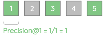
Similarly, precision@2 = 0.5 as only one of the top-2 results are relevant.

Thus, we can calculate the precision score for all k values.
| k | 1 | 2 | 3 | 4 | 5 |
|---|---|---|---|---|---|
| Precision@k | \(\frac{1}{1}=1\) | \(\frac{1}{2}=0.5\) | \(\frac{2}{3}=0.67\) | \(\frac{2}{4}=0.5\) | \(\frac{3}{5}=0.6\) |
A limitation of precision@k is that it doesn’t consider the position of the relevant items. Consider two models A and B that have the same number of relevant results i.e. 3 out of 5.
For model A, the first three items were relevant, while for model B, the last three items were relevant. Precision@5 would be the same for both of these models even though model A is better.

2. Recall@k
This metric gives how many actual relevant results were shown out of all actual relevant results for the query. Mathematically, this is given by:
\[ \text{Recall@k} = \frac{\text{true positives@k}}{(\text{true positives@k}) + (\text{false negatives@k})} \]
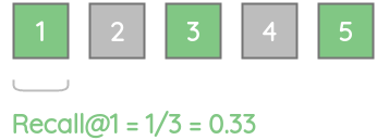
For our example, recall@1 = 0.33 as only one of the 3 actual relevant items are present.
Similarly, recall@3 = 0.67 as only two of the 3 actual relevant items are present.
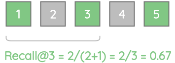
Thus, we can calculate the recall score for different K values.
| k | Recall@k |
|---|---|
| 1 | \(\frac{1}{(1+2)}=\frac{1}{3}=0.33\) |
| 2 | \(\frac{1}{(1+2)}=\frac{1}{3}=0.33\) |
| 3 | \(\frac{2}{(2+1)}=\frac{2}{3}=0.67\) |
| 4 | \(\frac{2}{(2+1)}=\frac{2}{3}=0.67\) |
| 5 | \(\frac{3}{(3+0)}=\frac{3}{3}=1\) |
3. F1@k
This is a combined metric that incorporates both Precision@k and Recall@k by taking their harmonic mean. We can calculate it as:
\[ \text{F1@k} = \frac{2*(\text{Precision@k}) * (\text{Recall@k})}{(\text{Precision@k}) + (\text{Recall@k})} \]
Using the previously calculated values of precision and recall, we can calculate F1-scores for different K values as shown below.
| Metric | Precision@k | Recall@k | F1@k |
|---|---|---|---|
| k=1 | 1 | 1/3 | \(\frac{2*1*(1/3)}{(1+1/3)}=0.5\) |
| k=2 | 1/2 | 1/3 | \(\frac{2*(1/2)*(1/3)}{(1/2+1/3)}=0.4\) |
| k=3 | 2/3 | 2/3 | \(\frac{2*(2/3)*(2/3)}{(2/3+2/3)}=0.666\) |
| k=4 | 1/2 | 2/3 | \(\frac{2*(1/2)*(2/3)}{(1/2+2/3)}=0.571\) |
| k=5 | 3/5 | 1 | \(\frac{2*(3/5)*1}{(3/5+1)}=0.749\) |
B. Order Aware Metrics
While precision, recall, and F1 give us a single-value metric, they don’t consider the order in which the returned search results are sent. To solve that limitation, people have devised order-aware metrics given below:
1. Mean Reciprocal Rank(MRR)
This metric is useful when we want our system to return the best relevant item and want that item to be at a higher position. Mathematically, this is given by:
\[ MRR = \frac{1}{|Q|} \sum_{i=1}^{|Q|} \frac{1}{rank_{i}} \]
where: - \(\lVert Q \rVert\) denotes the total number of queries
- \(rank_i\) denotes the rank of the first relevant result
To calculate MRR, we first calculate the reciprocal rank. It is simply the reciprocal of the rank of the first correct relevant result and the value ranges from 0 to 1.
For our example, the reciprocal rank is \(\frac{1}{1}=1\) as the first correct item is at position 1.
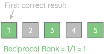
Let’s see another example where the only one relevant result is present at the end of the list i.e. position 5. It gets a lower reciprocal rank score of 0.2.

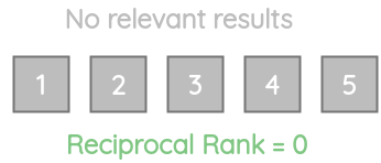
Let’s consider another example where none of the returned results are relevant. In such a scenario, the reciprocal rank will be 0.
For multiple different queries, we can calculate the MRR by taking the mean of the reciprocal rank for each query.
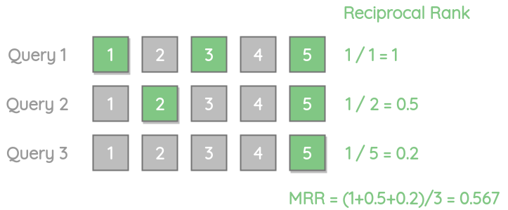
We can see that MRR doesn’t care about the position of the remaining relevant results. So, if your use-case requires returning multiple relevant results in the best possible way, MRR is not a suitable metric.
2. Average Precision(AP)
Average Precision is a metric that evaluates whether all of the ground-truth relevant items selected by the model are ranked higher or not. Unlike MRR, it considers all the relevant items.
Mathematically, it is given by:
\[ AP = \frac{\sum_{k=1}^{n} (P(k) * rel(k))}{\text{number of relevant items}} \]
where:
- \(rel(k)\) is an indicator function which is 1 when the item at rank K is relevant.
- \(P(k)\) is the Precision@k metric
For our example, we can calculate the AP based on our Precision@K values for different K.

\[ AP = \frac{(1 + 2/3 + 3/5)}{3} = 0.7555 \]
To illustrate the advantage of AP, let’s take our previous example but place the 3 relevant results at the beginning. We can see that this gets a perfect AP score than the above example.

\[ AP = \frac{(1 + 1 + 1)}{3} = 1 \]
3. Mean Average Precision(MAP)
If we want to evaluate average precision across multiple queries, we can use the MAP. It is simply the mean of the average precision for all queries. Mathematically, this is given by
\[ MAP = \frac{1}{Q} \sum_{q=1}^{Q} AP(q) \]
where
- \(Q\) is the total number of queries
- \(AP(q)\) is the average precision for query q.
Problem Setup 2: Graded Relevance
Let’s take another toy example where we annotated the items not just as relevant or not-relevant but instead used a grading scale between 0 to 5 where 0 denotes least relevant and 5 denotes the most relevant.
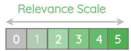
We have a ranking model that gives us back 5-most relevant results for a certain query. The first item had a relevance score of 3 as per our ground-truth annotation, the second item has a relevance score of 2 and so on.

Let’s understand the various metrics to evaluate this type of setup.
1. Cumulative Gain (CG@k)
This metric uses a simple idea to just sum up the relevance scores for top-K items. The total score is called cumulative gain. Mathematically, this is given by:
\[ CG@k = \sum_{1}^{k} rel_{i} \]
For our example, CG@2 will be 5 because we add the first two relevance scores 3 and 2.

Similarly, we can calculate the cumulative gain for all the K-values as:
| Position(k) | 1 | 2 | 3 | 4 | 5 |
|---|---|---|---|---|---|
| Cumulative Gain@k | 3 | 3+2=5 | 3+2+3=8 | 3+2+3+0=8 | 3+2+3+0+1=9 |
While simple, CG doesn’t take into account the order of the relevant items. So, even if we swap a less-relevant item to the first position, the CG@2 will be the same.

2. Discounted Cumulative Gain (DCG@k)
We saw how a simple cumulative gain doesn’t take into account the position. But, we would normally want items with a high relevance score to be present at a better rank.
Consider an example below. With the cumulative gain, we are simply adding the scores without taking into account their position.
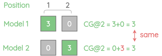
An item with a relevance score of 3 at position 1 is better than the same item with relevance score 3 at position 2.
So, we need some way to penalize the scores by their position. DCG introduces a log-based penalty function to reduce the relevance score at each position. For 5 items, the penalty would be
| \(\mathbf{i}\) | \(\mathbf{log_{2}(i+1)}\) |
|---|---|
| 1 | \(log_{2}(1+1) = log_{2}(2) = 1\) |
| 2 | \(log_{2}(2+1) = log_{2}(3) = 1.584\) |
| 3 | \(log_{2}(3+1) = log_{2}(4) = 2\) |
| 4 | \(log_{2}(4+1) = log_{2}(5) = 2.321\) |
| 5 | \(log_{2}(5+1) = log_{2}(6) = 2.584\) |
Using this penalty, we can now calculate the discounted cumulative gain simply by taking the sum of the relevance score normalized by the penalty. Mathematically, this is given by:
\[ DCG@k = \sum_{i=1}^{k} \frac{ \color{#81c784}{rel_{i}} }{ \color{#e57373}{log_{2}(i + 1)} } \]
To understand the behavior of the log-penalty, let’s plot ranking position in x-axis and the percentage of relevance score i.e. \(\frac{1}{log_{2}(i+1)} * 100\) in the y-axis. As seen, in position 1, we don’t apply any penalty and score remains unchanged. But, the percentage of score kept decays exponentially from 100% in position 1 to 63% in position 2, 50% in position 3, and so on.
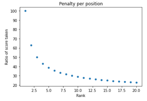
Let’s now calculate DCG for our example.

| \(\mathbf{Position(i)}\) | \(\mathbf{Relevance(rel_{i})}\) | \(\mathbf{log_{2}(i+1)}\) | \(\mathbf{\frac{rel_{i}}{log_{2}(i+1)}}\) |
|---|---|---|---|
| 1 | 3 | \(log_{2}(1+1) = log_{2}(2) = 1\) | \(\frac{3}{1} = 3\) |
| 2 | 2 | \(log_{2}(2+1) = log_{2}(3) = 1.5849\) | \(\frac{2}{1.5849} = 1.2618\) |
| 3 | 3 | \(log_{2}(3+1) = log_{2}(4) = 2\) | \(\frac{3}{2} = 1.5\) |
| 4 | 0 | \(log_{2}(4+1) = log_{2}(5) = 2.3219\) | \(\frac{0}{2.3219} = 0\) |
| 5 | 1 | \(log_{2}(5+1) = log_{2}(6) = 2.5849\) | \(\frac{1}{2.5849} = 0.3868\) |
Based on these penalized scores, we can now calculate DCG at various k values simply by taking their sum up to k.
| k | DCG@k |
|---|---|
| DCG@1 | \(3\) |
| DCG@2 | \(3+1.2618=4.2618\) |
| DCG@3 | \(3+1.2618+1.5=5.7618\) |
| DCG@4 | \(3+1.2618+1.5+0=5.7618\) |
| DCG@5 | \(3+1.2618+1.5+0+0.3868 = 6.1486\) |
There is also an alternative formulation for DCG@K that gives more penalty if relevant items are ranked lower. This formulation is preferred more in industry.
\[ DCG@k = \sum_{i=1}^{k} \frac{ \color{#81c784}{2^{rel_{i}} - 1} }{ \color{#e57373}{log_{2}(i + 1)} } \]
While DCG solves the issues with cumulative gain, it has a limitation. Suppose we a query Q1 with 3 results and query Q2 with 5 results. Then the query with 5 results Q2 will have a larger overall DCG score. But we can’t say that query 2 was better than query 1.

3. Normalized Discounted Cumulative Gain (NDCG@k)
To allow a comparison of DCG across queries, we can use NDCG that normalizes the DCG values using the ideal order of the relevant items.
Let’s take our previous example where we had already calculated the DCG values at various K values.

| k | DCG@k |
|---|---|
| DCG@1 | \(3\) |
| DCG@2 | \(3+1.2618=4.2618\) |
| DCG@3 | \(3+1.2618+1.5=5.7618\) |
| DCG@4 | \(3+1.2618+1.5+0=5.7618\) |
| DCG@5 | \(3+1.2618+1.5+0+0.3868 = 6.1486\) |
For our example, ideally, we would have wanted the items to be sorted in descending order of relevance scores.

Let’s calculate the ideal DCG(IDCG) for this order.
| \(\mathbf{Position(i)}\) | \(\mathbf{Relevance(rel_{i})}\) | \(\mathbf{log_{2}(i+1)}\) | \(\mathbf{\frac{rel_{i}}{log_{2}(i+1)}}\) | IDCG@k |
|---|---|---|---|---|
| 1 | 3 | \(log_{2}(2) = 1\) | 3 / 1 = 3 | 3 |
| 2 | 3 | \(log_{2}(3) = 1.5849\) | 3 / 1.5849 = 1.8927 | 3+1.8927=4.8927 |
| 3 | 2 | \(log_{2}(4) = 2\) | 2 / 2 = 1 | 3+1.8927+1=5.8927 |
| 4 | 1 | \(log_{2}(5) = 2.3219\) | 1 / 2.3219 = 0.4306 | 3+1.8927+1+0.4306=6.3233 |
| 5 | 0 | \(log_{2}(6) = 2.5849\) | 0 / 2.5849 = 0 | 3+1.8927+1+0.4306+0=6.3233 |
Now we can calculate the NDCG@k for various k by dividing DCG@k by IDCG@k as shown below:
\[ \text{NDCG@k} = \frac{\text{DCG@k}}{\text{IDCG@k}} \]
| \(k\) | DCG@k | IDCG@k | NDCG@k |
|---|---|---|---|
| 1 | 3 | 3 | \(\frac{3}{3} = 1\) |
| 2 | 4.2618 | 4.8927 | \(\frac{4.2618}{4.8927} = 0.8710\) |
| 3 | 5.7618 | 5.8927 | \(\frac{5.7618}{5.8927} = 0.9777\) |
| 4 | 5.7618 | 6.3233 | \(\frac{5.7618}{6.3233} = 0.9112\) |
| 5 | 6.1486 | 6.3233 | \(\frac{6.1486}{6.3233} = 0.9723\) |
Thus, we get NDCG scores with a range between 0 and 1. A perfect ranking would get a score of 1. We can also compare NDCG@k scores of different queries since it’s a normalized score.
Conclusion
Thus, we learned about various evaluation metrics for both binary and graded ground-truth labels and how each metric improves upon the previous.
References
Citation
@online{chaudhary2020,
  author = {Chaudhary, Amit},
  title = {Evaluation {Metrics} {For} {Information} {Retrieval}},
  date = {2020-08-04},
  url = {https://amitness.com/posts/information-retrieval-evaluation.html},
  langid = {en}
}