Unsupervised Keyphrase Extraction

Learn about unsupervised algorithms for automatically extracting representative keyword and phrases from documents

Keyword Extraction is one of the simplest ways to leverage text mining for providing business value. It can automatically identify the most representative terms in the document.

Such extracted keywords can be used for various applications. They can be used to summarize the underlying theme of a large document with just a few terms. They are also valuable as metadata for indexing and tagging the documents. They can likewise be used for clustering similar documents. For instance, to showcase relevant advertisements on a webpage, we could extract keywords from the webpage, find matching advertisements for these keywords, and showcase those.

In this post, I will provide an overview of the general pipeline of keyword extraction and explain the working mechanism of various unsupervised algorithms for this.

Unsupervised Keyphrase Extraction Pipeline

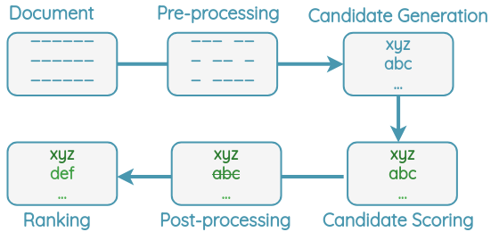
For keyword extraction, all algorithms follow a similar pipeline as shown below. A document is preprocessed to remove less informative words like stop words, punctuation, and split into terms. Candidate keywords such as words and phrases are chosen.

Then, a score is determined for each candidate keyword using some algorithm. The highest-ranking keywords are selected and post-processing such as removing near-duplicates is applied. Finally, the algorithm returns the top N ranking keywords as output.

Unsupervised Methods

Unsupervised algorithms for keyword extraction don’t need to be trained on the corpus and don’t need any pre-defined rules, dictionary, or thesaurus. They can use statistical features from the text itself and as such can be applied to large documents easily without re-training. Most of these algorithms don’t need any linguistic features except for stop word lists and so can be applied to multiple languages.

Let’s understand each algorithm by starting from simple methods and gradually adding complexity.

1. Naive Counting

This is a simple method which only takes into account how many times each term occurs.

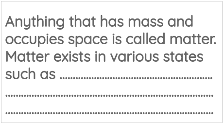
Let’s understand it by applying it to an example document.

a. Pre-processing

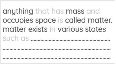
In this step, we lowercase the text and remove low informative words such as stop words from the text.

b. Candidate Generation

We split the remaining terms by space and punctuation symbols to get a list of possible keywords.

c. Candidate Scoring

We can count the number of times each term occurs to get a score for each term.

Candidate	anything	mass	occupies	space	called	matter	exists	various	states	…
Count	1	1	1	1	1	2	1	1	1	…

d. Final Ranking

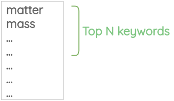
We can sort the keywords in descending order based on the counts and take the top N keywords as the output.

Drawback of Naive Counting

This method has an obvious drawback of only focusing on frequency. But, generic words are likely to be very frequent in any document but are not representative of the domain and topic of the document. We need some way to filter out generic terms.

2. Term Frequency Inverse Document Frequency (TF-IDF)

This method takes into account both how frequent the keyphrase is and also how rare it is across the documents.

Let’s understand how it works by going through the various steps of the pipeline:

a. Pre-processing

In this step, we lowercase the text and split the document into sentences.

b. Candidate Generation

We generate 1-gram, 2-gram, and 3-grams candidate phrases from each sentence such that they don’t contain any punctuations. These are our list of candidate phrases.

c. Candidate Scoring

Now, for each candidate keyword “w”, we calculate the TF-IDF score in the following steps.

First, the term frequency(TF) is calculated simply by counting the occurrence of the word.

\[ TF(w) = count(w) \]

Then, the inverse document frequency(IDF) is calculated by dividing the total number of documents by the number of documents that contain the word “w” and taking the log of that quantity.

\[ IDF(W) = log(\ \frac{total\ documents}{number\ of\ docs\ containing\ word\ w}\ ) \]

Finally, we get the TF-IDF score for a term by multiplying the two quantities.

\[ TFIDF(w) = TF(w) * IDF(w) \]

d. Final Ranking

We can sort the keywords in descending order based on their TF-IDF scores and take the top N keywords as the output.

3. Rapid Automatic Keyword Extraction (RAKE)

RAKE is a domain-independent keyword extraction method proposed in 2010. It uses word frequency and co-occurrence to identify the keywords. It is very useful for identifying relevant multi-word expressions.

How RAKE works

Let’s apply RAKE on a toy example document to understand how it works:

a. Preprocessing

First, the stop words in the document are removed.

b. Candidate Generation

We split the document at the stop word positions and punctuations to get content words. The words that occur consecutively without any stop word between them are taken as candidate keywords.

For example, “Deep Learning” is treated as a single keyword.

c. Candidate Scoring

Next, the frequency of all the individual words in the candidate keywords are calculated. This finds words that occur frequently.

	deep	learning	subfield	ai	useful
Word Frequency: \(freq(w)\)	1	1	1	1	1

Similarly, the word co-occurrence count is calculated and the degree for each word is the total sum. This metric identifies words that occur often in longer candidate keywords.

	deep	learning	subfield	ai	useful
deep	1	1	0	0	0
learning	1	1	0	0	0
subfield	0	0	1	0	0
ai	0	0	0	1	0
useful	0	0	0	0	1
degree: \(deg(w)\)	1 + 1 = 2	1 + 1 = 2	1	1	1

Then, we divide the degree by the frequency for each word to get a final score. This score identifies words that occur more in longer candidate keywords than individually.

	deep	learning	subfield	ai	useful
Score = \(\frac{deg(w)}{freq(w)}\)	2 / 1 = 2	2 / 1 = 2	1 / 1 = 1	1 / 1 = 1	1 / 1 = 1

d. Final Ranking

Finally, we calculate the scores for our candidate keywords by adding the scores for their member words. The higher the score, the more useful a keyword is.

Keyword	Score	Remarks
deep learning	4	score(deep) + score(learning) = 2 + 2 = 4
subfield	1	score(subfield) = 1
ai	1	score(ai) = 1
useful	1	score(useful) = 1

Thus, the keywords are sorted in the descending order of their score value. We can select the top-N keywords from this list.

Drawbacks of RAKE

• If the stop word list used in RAKE is not exhaustive, it would treat continuous long text as a phrase and give very long phrases.
• Multi-word expressions that contain stop-words could be missed. For example, mention of a brand called “Good Day” could be missed if “good” is present in the stop word list.

Using RAKE in Python

We can use the rake-nltk library to use it in Python as shown below.

pip install rake-nltk

from rake_nltk import Rake
rake = Rake()

text = 'Deep Learning is a subfield of AI. It is very useful.'
rake.extract_keywords_from_text(text)

print(rake.get_ranked_phrases_with_scores())

[(4.0, 'deep learning'), (1.0, 'useful'), (1.0, 'subfield'), (1.0, 'ai')]

4. Yet Another Keyword Extractor (YAKE)

YAKE is another popular keyword extraction algorithm proposed in 2018. It outperforms TF-IDF and RAKE across many datasets and went on to win the best “short paper award” at ECIR 2018.

YAKE uses statistical features to identify and rank the most important keywords. It doesn’t need any linguistic information like NER or POS tagging and thus can be used with any language. It only requires a stop word list for the language.

How YAKE works:

i. Preprocessing and Candidate Generation

The sentences are split into terms using space and special character(line break, bracket, comma, period) as the delimiter.

We decide the maximum length of the keyword to be generated. If we decide max length of 3, then 1-gram, 2-gram, and 3-gram candidate phrases are generated using a sliding window.

Then, we remove phrases that contain punctuation marks. Also, phrases that begin and end with a stop word are removed.

ii. Candidate Scoring

YAKE uses 5 features to quantify how good each word is.

a. Casing

This feature considers the casing of the word. It gives more importance to capitalized words and acronyms such as “NASA”.

First, we count the number of times the word starts with a capital letter when it is not the beginning word of the sentence. We also count the times when the word is in acronym form.

Then, we take the maximum of the two counts and normalize it by the log of the total count.

\[ casing(w) = \frac{max( count(w\ is\ capital), count(w\ is\ acronym) )}{1 + log(count(w))} \]

b. Word Positional

This feature gives more importance to words present at the beginning of the document. It’s based on the assumption that relevant keywords are usually concentrated more at the beginning of a document.

First, we get all the sentence positions where the word “w” occurs.

\[ Sen(w) = positions\ of\ sentences\ where\ w\ occurs \]

Then, we compute the position feature by taking the median position and applying the following formula:

\[ position(w) = log( log( 3 + Median(Sen(w)) ) ) \]

c. Word Frequency

This feature calculates the frequency of the words normalized by 1-standard deviation from the mean.

\[ frequency(w) = \frac{count\ of\ word\ w}{mean(counts) + standard\ deviation(counts)} \]

d. Word Relatedness to Context

This feature quantifies how related a word is to its context. For that, it counts how many different terms occur to the left or right of a candidate word. If the word occurs frequently with different words on the left or right side, it is more likely to be a stop word.

\[ relatedness(w) = 1 + (WR + WL) * \frac{count(w)}{max\ count} + PL + PR \]

where,

• WR = (number of unique words on right) / (total words on right)
• WL = (number of unique words on left) / (total words on left)
• PL = (total words on left) / (max count)
• PR = (total words on right) / (max count)

e. Word Different Sentence

This feature quantifies how often a candidate word occurs with different sentences. A word that often occurs in different sentences has a higher score.

\[ different(w) = \frac{number\ of\ sentences\ w\ occurs\ in}{total\ sentences} \]

Combined Word Score

These 5 features are combined into a single score S(w) using the formula:

\[ score(w) = \frac{d * b}{a + (c / d) + (e / d)} \]

where,

• a = casing
• b = position
• c = frequency
• d = relatedness
• e = different

Keyword Score

Now, for each of our candidate keywords, a score is calculated using the following formula. The count of keyword penalizes less frequent keywords.

\[ S(kw) = \frac{product(scores\ of\ words\ in\ keyword)}{1 + (sum\ of\ scores\ of\ words) * count(keyword)} \]

iii. Post-processing

It’s pretty common to get similar candidates when extracting keyphrases. For example, we could have variations like:

• “work”, “works”
  
• “relevant”, “relevance”

To eliminate such duplicates, the following process is applied:

• First, the keywords are sorted in ascending order of their scores and we maintain a list of chosen keywords so far
  
• Then, for each keyword in the list
  • If the keyword has a small Levenshtein distance with any of chosen keywords so far, it is skipped
  • Otherwise, the keyword is added to the chosen keywords list

Thus, the chosen keyword list contains the final deduplicated keywords.

iv. Final Ranking

Thus, we have a list of keywords along with their scores. A keyword is more important if it has a lower score.

We can sort the keywords in ascending order and take the top N keywords as the output.

Using YAKE in Python

To apply YAKE, we will use the pke library. First, we need to install the library and its dependencies using the following command:

pip install git+https://github.com/boudinfl/pke.git
python -m nltk.downloader stopwords
python -m spacy download en

Then, we can use YAKE to generate keywords of maximum length 2 as shown below.

from pke.unsupervised import YAKE
from nltk.corpus import stopwords

document = "Machine learning (ML) is the study of computer algorithms that improve automatically through experience. It is seen as a subset of artificial intelligence."

# 1. Create YAKE keyword extractor
extractor = YAKE()

# 2. Load document
extractor.load_document(input=document,
                        language='en',
                        normalization=None)


# 3. Generate candidate 1-gram and 2-gram keywords
stoplist = stopwords.words('english')
extractor.candidate_selection(n=2, stoplist=stoplist)

# 4. Calculate scores for the candidate keywords
extractor.candidate_weighting(window=2,
                              stoplist=stoplist,
                              use_stems=False)

# 5. Select 10 highest ranked keywords
# Remove redundant keywords with similarity above 80%
key_phrases = extractor.get_n_best(n=10, threshold=0.8)
print(key_phrases)

You get back a list of top-10 keywords and their scores. The highest ranked keyword has the lowest score.

[('machine learning', 0.01552184797949213),
 ('computer algorithms', 0.04188746641162499),
 ('improve automatically', 0.04188746641162499),
 ('machine', 0.12363091320521931),
 ('learning', 0.12363091320521931),
 ('experience', 0.12363091320521931),
 ('artificial intelligence', 0.18075564686791562),
 ('study', 0.2005079697193566),
 ('computer', 0.2005079697193566),
 ('algorithms', 0.2005079697193566)]

References

• Rose, Stuart & Engel, Dave & Cramer, Nick & Cowley, Wendy. (2010). Automatic Keyword Extraction from Individual Documents.10.1002/9780470689646.ch1
• Eirini Papagiannopoulou et al., “A Review of Keyphrase Extraction”
• “YAKE implementation in pke: an open source python-based keyphrase extraction toolkit”