Semi-Supervised Learning in Computer Vision
Semi-supervised learning methods for Computer Vision have been advancing quickly in the past few years. Current state-of-the-art methods are simplifying prior work in terms of architecture and loss function or introducing hybrid methods by blending different formulations.
In this post, I will illustrate the key ideas of these recent methods for semi-supervised learning through diagrams.
1. Self-Training
In this semi-supervised formulation, a model is trained on labeled data and used to predict pseudo-labels for the unlabeled data. The model is then trained on both ground truth labels and pseudo-labels simultaneously.

a. Pseudo-label
Lee (2013) proposed a very simple and efficient formulation called “Pseudo-label” in 2013.
The idea is to train a model simultaneously on a batch of both labeled and unlabeled images. The model is trained on labeled images in usual supervised manner with a cross-entropy loss. The same model is used to get predictions for a batch of unlabeled images and the maximum confidence class is used as the pseudo-label. Then, cross-entropy loss is calculated by comparing model predictions and the pseudo-label for the unlabeled images .
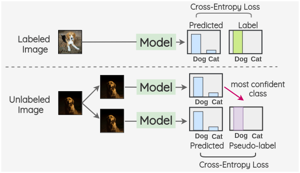
The total loss is a weighted sum of the labeled and unlabeled loss terms.
\[ L = L_{labeled} + \alpha_{t} * L_{unlabeled} \]
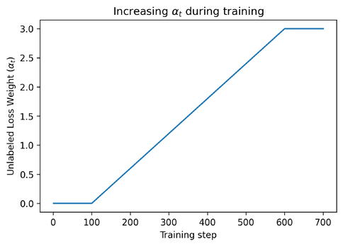
To make sure the model has learned enough from the labeled data, the \(\alpha_t\) term is set to 0 during the initial 100 training steps. It is then gradually increased up to 600 training steps and then kept constant.
b. Noisy Student
Xie et al. (2019b) proposed a semi-supervised method inspired by Knowledge Distillation called “Noisy Student” in 2019.
The key idea is to train two separate models called “Teacher” and “Student”. The teacher model is first trained on the labeled images and then it is used to infer the pseudo-labels for the unlabeled images. These pseudo-labels can either be soft-label or converted to hard-label by taking the most confident class. Then, the labeled and unlabeled images are combined together and a student model is trained on this combined data. The images are augmented using RandAugment as a form of input noise. Also, model noise such as Dropout and Stochastic Depth are incorporated in the student model architecture.
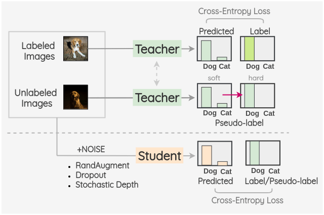
Once a student model is trained, it becomes the new teacher and this process is repeated for three iterations.
2. Consistency Regularization
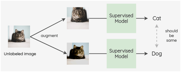
This paradigm uses the idea that model predictions on an unlabeled image should remain the same even after adding noise. We could use input noise such as Image Augmentation and Gaussian noise. Noise can also be incorporated in the architecture itself using Dropout.
a. π-model
This model was proposed by Laine and Aila (2017) in a conference paper at ICLR 2017.
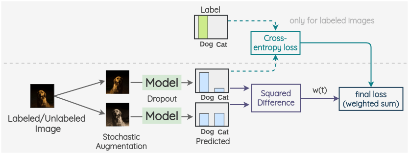
The key idea is to create two random augmentations of an image for both labeled and unlabeled data. Then, a model with dropout is used to predict the label of both these images. The square difference of these two predictions is used as a consistency loss. For labeled images, we also calculate the cross-entropy loss. The total loss is a weighted sum of these two loss terms. A weight w(t) is applied to decide how much the consistency loss contributes in the overall loss.
b. Temporal Ensembling
This method was also proposed by Laine and Aila (2017) in the same paper as the pi-model. It modifies the π-model by leveraging the Exponential Moving Average(EMA) of predictions.
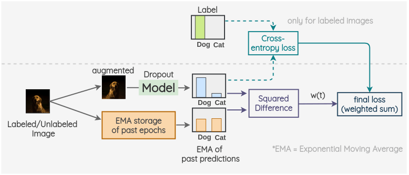
The key idea is to use the exponential moving average of past predictions as one view. To get another view, we augment the image as usual and a model with dropout is used to predict the label. The square difference of current prediction and EMA prediction is used as a consistency loss. For labeled images, we also calculate the cross-entropy loss. The final loss is a weighted sum of these two loss terms. A weight w(t) is applied to decide how much the consistency loss contributes in the overall loss.
c. Mean Teacher
This method was proposed by Tarvainen and Valpola (2017). The general approach is similar to Temporal Ensembling but it uses Exponential Moving Average(EMA) of the model parameters instead of predictions.
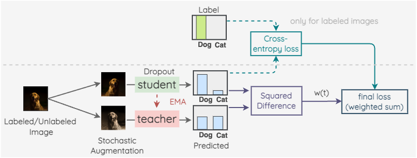
The key idea is to have two models called “Student” and “Teacher”. The student model is a regular model with dropout. And the teacher model has the same architecture as the student model but its weights are set using an exponential moving average of the weights of student model. For a labeled or unlabeled image, we create two random augmented versions of the image. Then, the student model is used to predict label distribution for first image. And, the teacher model is used to predict the label distribution for the second augmented image. The square difference of these two predictions is used as a consistency loss. For labeled images, we also calculate the cross-entropy loss. The final loss is a weighted sum of these two loss terms. A weight w(t) is applied to decide how much the consistency loss contributes in the overall loss.
d. Virtual Adversarial Training
This method was proposed by Miyato et al. (2019). It uses the concept of adversarial attack for consistency regularization.
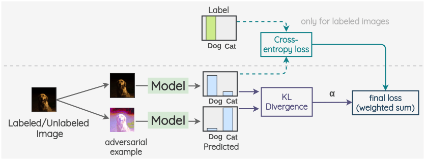
The key idea is to generate an adversarial transformation of an image that will change the model prediction. To do so, first, an image is taken and an adversarial variant of it is created such that the KL-divergence between the model output for the original image and the adversarial image is maximized.
Then we proceed as previous methods. We take a labeled/unlabeled image as first view and take its adversarial example generated in previous step as the second view. Then, the same model is used to predict label distributions for both images. The KL-divergence of these two predictions is used as a consistency loss. For labeled images, we also calculate the cross-entropy loss. The final loss is a weighted sum of these two loss terms. A weight \(\alpha\) is applied to decide how much the consistency loss contributes in the overall loss.
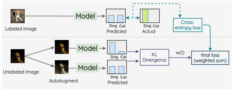
e. Unsupervised Data Augmentation
This method was proposed by Xie et al. (2019a) and works for both images and text. Here, we will understand the method in the context of images.
The key idea is to create an augmented version of a unlabeled image using AutoAugment. Then, a same model is used to predict the label of both these images. The KL-divergence of these two predictions is used as a consistency loss. For labeled images, we only calculate the cross-entropy loss and don’t calculate any consistency loss. The final loss is a weighted sum of these two loss terms. A weight w(t) is applied to decide how much the consistency loss contributes in the overall loss.
3. Hybrid Methods
This paradigm combines ideas from previous work such as self-training and consistency regularization along with additional components for performance improvement.
a. MixMatch
This holistic method was proposed by Berthelot et al. (2019).
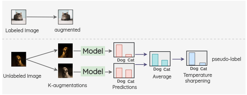
To understand this method, let’s take a walk through each of the steps.
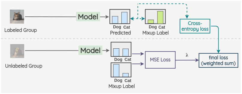
For the labeled image, we create an augmentation of it. For the unlabeled image, we create K augmentations and get the model predictions on all K-images. Then, the predictions are averaged and temperature scaling is applied to get a final pseudo-label. This pseudo-label will be used for all the K-augmentations.
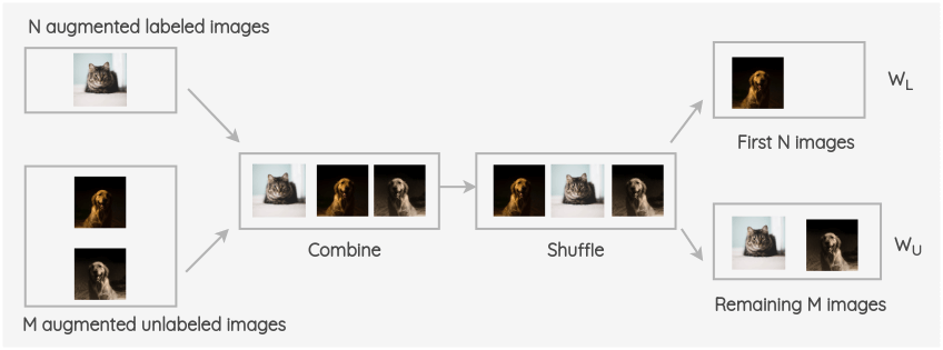
The batches of augmented labeled and unlabeled images are combined and the whole group is shuffled. Then, the first N images of this group are taken as \(W_L\), and the remaining M images are taken as \(W_U\).
Now, Mixup is applied between the augmented labeled batch and group \(W_L\). Similarly, mixup is applied between the M augmented unlabeled group and the \(W_U\) group. Thus, we get the final labeled and unlabeled group.
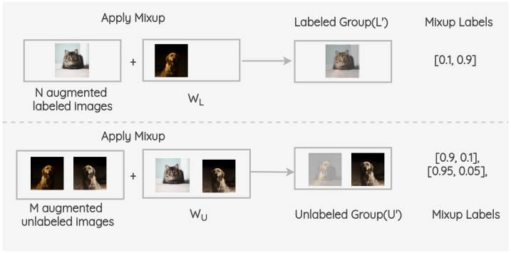
Now, for the labeled group, we take model predictions and compute cross-entropy loss with the ground truth mixup labels. Similarly, for the unlabeled group, we compute model predictions and compute mean square error(MSE) loss with the mixup pseudo labels. A weighted sum is taken of these two terms with \(\lambda\) weighting the MSE loss.
b. FixMatch
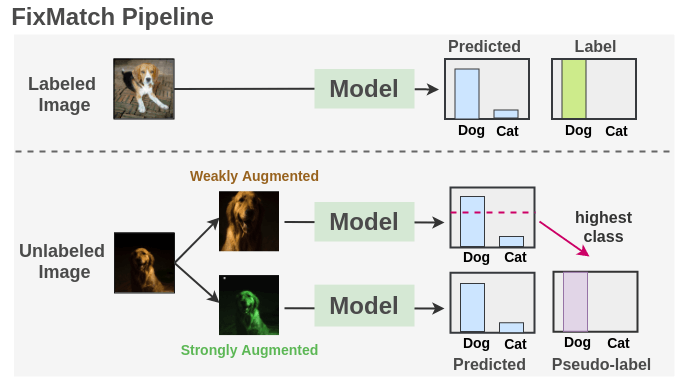
This method was proposed by Sohn et al. (2020) and combines pseudo-labeling and consistency regularization while vastly simplifying the overall method. It got state of the art results on a wide range of benchmarks.
As seen, we train a supervised model on our labeled images with cross-entropy loss. For each unlabeled image, weak augmentation and strong augmentations are applied to get two images. The weakly augmented image is passed to our model and we get prediction over classes. The probability for the most confident class is compared to a threshold. If it is above the threshold, then we take that class as the ground label i.e. pseudo-label. Then, the strongly augmented image is passed through our model to get a prediction over classes. This prediction is compared to ground truth pseudo-label using cross-entropy loss. Both the losses are combined and the model is optimized.
If you want to learn more about FixMatch, I have an article that goes over it in depth.
Comparison of Methods
Here is a high-level summary of the differences between all the above-mentioned methods.
| Method Name | Year | Unlabeled Loss | Augmentation |
|---|---|---|---|
| Pseudo-label | 2013 | Cross-Entropy | Random |
| π-model | 2016 | MSE | Random |
| Temporal Ensembling | 2016 | MSE | Random |
| Mean Teacher | 2017 | MSE | Random |
| Virtual Adversarial Training(VAT) | 2017 | KL-divergence | Adversarial transformation |
| Unsupervised Data Augmentation(UDA) | 2019 | KL-divergence | AutoAugment |
| MixMatch | 2019 | MSE | Random |
| Noisy Student | 2019 | Cross-Entropy | RandAugment |
| FixMatch | 2020 | Cross-Entropy | CTAugment / RandAugment |
Common Evaluation Datasets
To evaluate the performance of these semi-supervised methods, the following datasets are commonly used. The authors simulate a low-data regime by using only a small portion(e.g. 40/250/4000/10000 examples) of the whole dataset as labeled and treating the remaining as the unlabeled set.
| Dataset | Classes | Image Size | Train | Validation | Unlabeled |
|---|---|---|---|---|---|
| CIFAR-10 | 10 | 32*32 | 50,000 | 10,000 | - |
| CIFAR-100 | 100 | 32*32 | 50,000 | 10,000 | - |
| STL-10 | 10 | 96*96 | 5000 | 8000 | 1,00,000 |
| SVHN | 10 | 32*32 | 73,257 | 26,032 | 5,31,131 |
| ILSVRC-2012 | 1000 | vary | 1.2 million | 150,000 | 1,50,000 |
Conclusion
Thus, we got an overview of how semi-supervised methods for Computer Vision have progressed over the years. This is a really important line of research that can have a direct impact on the industry.
References
Citation
@online{chaudhary2020,
  author = {Chaudhary, Amit},
  title = {Semi-Supervised {Learning} in {Computer} {Vision}},
  date = {2020-07-12},
  url = {https://amitness.com/posts/semi-supervised-learning.html},
  langid = {en}
}