The Illustrated FixMatch for Semi-Supervised Learning
Deep Learning has shown very promising results in the area of Computer Vision. But when applying it to practical domains such as medical imaging, lack of labeled data is a major hurdle.
In practical settings, labeling data is a time consuming and expensive process. Though, you have a lot of images, only a small portion of them can be labeled due to resource constraints. In such settings, we could wonder:
How can we leverage the remaining unlabeled images along with the labeled images to improve the performance of our model?
The answer lies in a field called semi-supervised learning. FixMatch is a recent semi-supervised approach by Sohn et al. (2020) from Google Brain that improved the state of the art in semi-supervised learning(SSL). It is a simpler combination of previous methods such as UDA and ReMixMatch.
In this post, we will understand FixMatch and also see how it got 78% median accuracy and 84% maximum accuracy on CIFAR-10 with just 10 labeled images.
Intuition behind FixMatch
Suppose we’re doing a cat vs dog classification where we have limited labeled data and a lot of unlabelled images of cats and dogs.
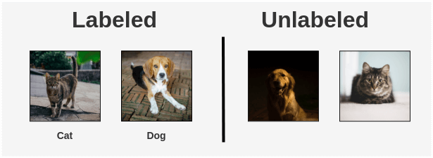
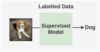
Our usual supervised learning approach would be to just train a classifier on labeled images and ignore the unlabelled images.
We know that a model should be able to handle perturbations of an image to improve generalization. So, instead of ignoring unlabeled images, we could instead apply the below approach:
What if we create augmented versions of unlabeled images and make the supervised model predict those images. Since it’s the same image, the predicted labels should be the same for both.
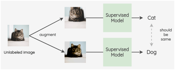
Thus, even without knowing their correct labels, we can use the unlabeled images as a part of our training pipeline. This is the core idea behind FixMatch and many preceding papers it builds upon.
The FixMatch Pipeline
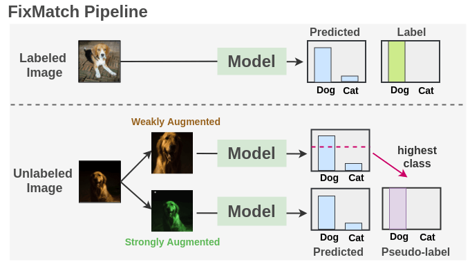
With the intuition clear, let’s see how FixMatch is applied in practice. The overall pipeline is summarized by the following figure:
Synopsis:
As seen, we train a supervised model on our labeled images with cross-entropy loss. For each unlabeled image, weak augmentation and strong augmentations are applied to get two images. The weakly augmented image is passed to our model and we get prediction over classes.
The probability for the most confident class is compared to a threshold. If it is above the threshold, then we take that class as the ground label i.e. pseudo-label. Then, the strongly augmented image is passed through our model to get a prediction over classes. This probability distribution is compared to ground truth pseudo-label using cross-entropy loss. Both the losses are combined and the model is tuned.
1. Training Data and Augmentation
FixMatch borrows this idea from UDA and ReMixMatch to apply different augmentation i.e weak augmentation on unlabeled image for the pseudo-label generation and strong augmentation on unlabeled image for prediction.
a. Weak Augmentation
For weak augmentation, the paper uses a standard flip-and-shift strategy. It includes two simple augmentations:
i. Random Horizontal Flip

This augmentation is applied with a probability of 50%. This is skipped for the SVHN dataset since those images contain digits for which horizontal flip is not relevant. In PyTorch, this can be performed using transforms as:
from PIL import Image
import torchvision.transforms as transforms

im = Image.open('dog.png')
weak_im = transforms.RandomHorizontalFlip(p=0.5)(im)
ii. Random Vertical and Horizontal Translation

This augmentation is applied up to 12.5%. In PyTorch, this can be implemented using the following code where 32 is the size of the image needed:
import torchvision.transforms as transforms
from PIL import Image

im = Image.open('dog.png')
resized_im = transforms.Resize(32)(im)
translated = transforms.RandomCrop(size=32,
                                    padding=int(32*0.125),
                                    padding_mode='reflect')(resized_im)
b. Strong Augmentation
These include augmentations that output heavily distorted versions of the input images. FixMatch applies either RandAugment or CTAugment and then applies CutOut augmentation.
1. Cutout
This augmentation randomly removes a square part of the image and fills it with gray or black color.

PyTorch doesn’t have a built-in implementation of Cutout but we can reuse its RandomErasing transformation to apply the CutOut effect.
import torch
import torchvision.transforms as transforms

# Image of 520*520
im = torch.rand(3, 520, 520)

# Fill cutout with gray color
gray_code = 127

# ratio=(1, 1) to set aspect ratio of square
# p=1 means probability is 1, so always apply cutout
# scale=(0.01, 0.01) means we want to get cutout of 1% of image area
# Hence: Cuts out gray square of 52*52
cutout_im = transforms.RandomErasing(p=1,
                                     ratio=(1, 1),
                                     scale=(0.01, 0.01),
                                     value=gray_code)(im)
2. AutoAugment Variants
Previous SSL work used AutoAugment, which trained a Reinforcement Learning algorithm to find augmentations that leads to the best accuracy on a proxy task(e.g. CIFAR-10). This is problematic since we require some labeled dataset to learn the augmentation and also due to resource requirements associated with RL.
So, FixMatch uses one among two variants of AutoAugment:
a. RandAugment
The idea of Random Augmentation(RandAugment) is very simple.
- First, you have a list of 14 possible augmentations with a range of their possible magnitudes.

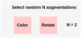
- You select random N augmentations from this list. Here, we are selecting any two from the list.
- Then you select a random magnitude M ranging from 1 to 10. We can select a magnitude of 5. This means a magnitude of 50% in terms of percentage as maximum possible M is 10 and so percentage = 5/10 = 50%.
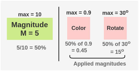
- Now, the selected augmentations are applied to an image in the sequence. Each augmentation has a 50% probability of being applied.

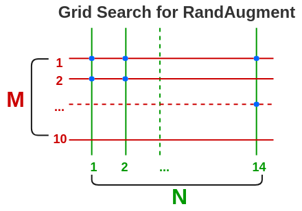
- The values of N and M can be found by hyper-parameter optimization on a validation set with a grid search. In the paper, they use random magnitude from a pre-defined range at each training step instead of a fixed magnitude.
b. CTAugment
CTAugment was an augmentation technique introduced in the ReMixMatch paper and uses ideas from control theory to remove the need for Reinforcement Learning in AutoAugment. Here’s how it works:
- We have a set of 18 possible transformations similar to RandAugment
- Magnitude values for transformations are divided into bins and each bin is assigned a weight. Initially, all bins weigh 1.
- Now two transformations are selected at random with equal chances from this set and their sequence forms a pipeline. This is similar to RandAugment.
- For each transformation, a magnitude bin is selected randomly with a probability according to the normalized bin weights
- Now, a labeled example is augmented with these two transformations and passed to the model to get a prediction
- Based on how close the model predictions were to the actual label, the magnitude bins weights for these transformations are updated.
- Thus, it learns to choose augmentations that the model has a high chance to predict a correct label and thus augmentation that fall within the network tolerance.
Thus, we see that unlike RandAugment, CTAugment can learn magnitude for each transformation dynamically during training. So, we don’t need to optimize it on some supervised proxy task and it has no sensitive hyperparameters to optimize.
Thus, this is very suitable for the semi-supervised setting where labeled data is scarce.
2. Model Architecture
The paper uses wider and shallower variants of ResNet called “Wide Residual Networks” (Zagoruyko and Komodakis, 2016) as the base architecture.
The exact variant used is Wide-Resnet-28-2 with a depth of 28 and a widening factor of 2. This model is two times wider than the ResNet. It has a total of 1.5 million parameters. The model is stacked with an output layer with nodes equal to the number of classes needed(e.g. 2 classes for cat/dog classification).
3. Model Training and Loss Function
Step 1: Preparing batches
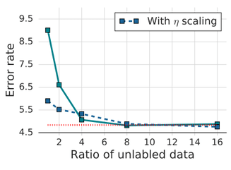
We prepare batches of the labeled images of size B and unlabeled images of batch size \(\color{#774cc3}{\mu} B\). Here \(\color{#774cc3}{\mu}\) is a hyperparameter that decides the relative size of labeled: unlabeled images in a batch. For example, \(\color{#774cc3}{\mu}=2\) means that we use twice the number of unlabeled images compared to labeled images.
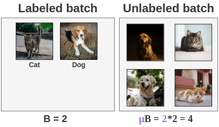
The paper tried increasing values of \(\color{#774cc3}{\mu}\) and found that as we increased the number of unlabeled images, the error rate decreases. The paper uses \(\color{#774cc3}{\mu} = 7\) for evaluation datasets.
Step 2: Supervised Learning
For the supervised part of the pipeline which is trained on labeled images, we use the regular cross-entropy loss H() for classification task. The total loss for a batch is defined by \(l_s\) and is calculated by taking average of cross-entropy loss for each image in the batch.

\[ l_s = \frac{1}{B} \sum_{b=1}^{B} \color{#9A0007}{H(}\ \color{#7ead16}{p_{b}}, \color{#5CABFD}{p_{m}(}\ y\ | \color{#FF8A50}{\alpha(} \color{#8c5914}{x_b} \color{#FF8A50}{)}\ \color{#5CABFD}{)} \color{#9A0007}{)} \]
Step 3: Pseudolabeling
For the unlabeled images, first we apply weak augmentation to the unlabeled image and get the highest predicted class by applying argmax. This is the pseudo-label that will be compared with output of model on strongly augmented image.
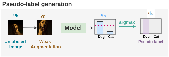
\[ \color{#5CABFD}{q_b} = p_m(y | \color{#8C5914}{\alpha(} \color{#007C91}{u_b} \color{#8C5914}{)} ) \]
\[ \color{#866694}{\hat{q_b}} = \color{#48A999}{argmax(}\color{#5CABFD}{q_b} \color{48A999}{)} \]
Step 4: Consistency Regularization
Now, the same unlabeled image is strongly augmented and it’s output is compared to our pseudolabel to compute cross-entropy loss H(). The total unlabeled batch loss is denoted by \(l_u\) and given by:
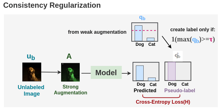
\[ l_u = \frac{1}{\mu B} \sum_{b=1}^{\mu B} 1(max(q_b) >= \color{#d11e77}{\tau})\ \color{#9A0007}{H(} \color{#866694}{\hat{q_b}}, p_m(y | \color{#25561F}{A(} \color{#007C91}{u_b} \color{#25561F}{)} \ \color{#9A0007}{)} \]
Here \(\color{#d11e77}{\tau}\) denotes the threshold above which we take a pseudo-label. This loss is similar to the pseudo-labeling loss. The difference is that we’re using weak augmentation to generate labels and strong augmentation for loss.
Step 5: Curriculum Learning
We finally combine these two losses to get a total loss that we optimize to improve our model. \(\lambda_u\) is a fixed scalar hyperparameter that decides how much both the unlabeled image loss contribute relative to the labeled loss.
\[ loss = l_s + \lambda_u l_u \]
An interesting result comes from \(\lambda_u\). Previous works have shown that increasing weight during training is good. But, in FixMatch, this is present in the algorithm itself.
Since initially, the model is not confident on labeled data, so its output predictions on unlabeled data will be below the threshold. As such, the model will be trained only on labeled data. But as the training progress, the model becomes more confident in labeled data and as such, predictions on unlabeled data will also start to cross the threshold. As such, the loss will soon start incorporating predictions on unlabeled images as well. This gives us a free form of curriculum learning.
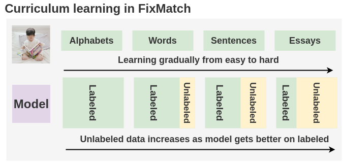
Intuitively, this is similar to how we’re taught in childhood. In the early years, we learn easy concepts such as alphabets and what they represent before moving on to complex topics like word formation, sentence formation, and then essays.
Paper Insights
Q. Can we learn with just one image per class?
The authors performed a really interesting experiment on the CIFAR-10 dataset. They trained a model on CIFAR-10 using only 10 labeled images i.e. 1 labeled example of each class.
They created 4 datasets by randomly selecting 1 example per class from the dataset and trained on each dataset 4 times. They reached a test accuracy between 48.58% to 85.32% with a median accuracy of 64.28%. This variability in the accuracy was caused due to the quality of labeled examples. It is difficult for a model to learn each class effectively when provided with low-quality examples.
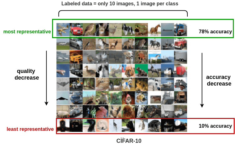
To test this, they created 8 training datasets with examples ranging from most representative to the least representative. They followed the ordering from Carlini et al. (2019) and created 8 buckets. The first bucket would contain the most representative images while the last bucket would contain outliers. Then, they took one example of each class randomly from each bucket to create 8 labeled training sets and trained the FixMatch model.
Results were:
- Most representative bucket: 78% median accuracy with a maximum accuracy of 84%
- Middle bucket: 65% accuracy
- Outlier bucket: Fails to converge completely with only 10% accuracy
Evaluation and Results
The authors ran evaluations on datasets commonly used for SSL such as CIFAR-10, CIFAR-100, SVHN, STL-10, and ImageNet.
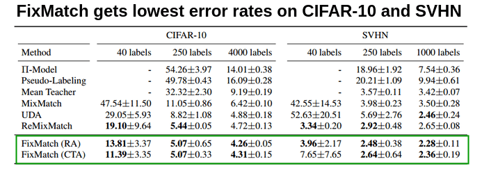
CIFAR-10 and SVHN:
FixMatch achieves the state of the art results on CIFAR-10 and SVHN benchmarks. They use 5 different folds for each dataset.
CIFAR-100
On CIFAR-100, ReMixMatch is a bit superior to FixMatch. To understand why the authors borrowed various components from ReMixMatch to FixMatch and measured their impact on performance.
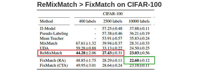
They found that the Distribution Alignment(DA) component which encourages the model to emit all classes with equal probability was the cause. So, when they combined FixMatch with DA, they achieved a 40.14% error rate compared to a 44.28% error rate of ReMixMatch.
STL-10
STL-10 dataset consists of 100,000 unlabeled images and 5000 labeled images. We need to predict 10 classes(airplane, bird, car, cat, deer, dog, horse, monkey, ship, truck.). It is a more representative evaluation for semi-supervised learning because its unlabeled set has out-of-distribution images.

FixMatch achieves the lowest error rate with CTAugment when evaluated on 5-folds of 1000 labeled images each among all methods.
ImageNet
The authors also evaluate the model on ImageNet to verify if it works on large and complex datasets. They take 10% of the training data as labeled images and all remaining 90% as unlabeled. Also, the architecture used is ResNet-50 instead of WideResNet and RandAugment is used as a strong augmentation.
They achieve a top-1 error rate of \(28.54\pm0.52%\) which is \(2.68\%\) better than UDA. The top-5 error rate is \(10.87\pm0.28\%\).
Code Implementation
The official implementation of FixMatch in Tensorflow by the paper authors is available here.
Unofficial implementations of FixMatch paper in PyTorch are available on GitHub (first, second, third). They use RandAugment and are evaluated on CIFAR-10 and CIFAR-100.
The paper is available here: FixMatch on Arxiv.
References
Citation
@online{chaudhary2020,
  author = {Chaudhary, Amit},
  title = {The {Illustrated} {FixMatch} for {Semi-Supervised}
    {Learning}},
  date = {2020-03-31},
  url = {https://amitness.com/posts/fixmatch.html},
  langid = {en}
}