The Illustrated PIRL: Pretext-Invariant Representation Learning
The end of 2019 saw a huge surge in the number of self-supervised learning research papers using contrastive learning. In December 2019, Misra et al. from Facebook AI Research proposed a new method PIRL (pronounced as “pearl”) for learning image representations.
In this article, I will explain the rationale behind the paper and how it advances the self-supervised representation learning scene further for images. We will also see how this compares to the current SOTA approach “SimCLR” (as of March 16, 2020) which improves shortcomings of PIRL.
Motivation
A number of interesting self-supervised learning methods have been proposed to learn image representations in recent times. Many of these use the idea of setting up a pretext task exploiting some geometric transformation to get labels. This includes Geometric Rotation Prediction, Context Prediction, Jigsaw Puzzle, Frame Order Recognition, Auto-Encoding Transformation (AET) among many others.

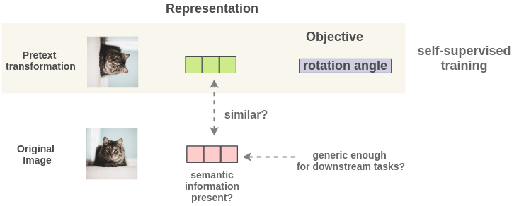
The pretext task is set up such that representations are learned for a transformed image to predict some property of transformation. For example, for a rotation prediction task, we randomly rotate the image by say 90 degrees and then ask the network to predict the rotation angle.

As such, the image representations learned can overfit to this objective of rotation angle prediction and not generalize well on downstream tasks. The representations will be covariant with the transformation. It will only encode essential information to predict rotation angle and could discard useful semantic information.
The PIRL Concept
PIRL proposes a method to tackle the problem of representations being covariant with transformation. It proposes a problem formulation such that representations generated for both the original image and transformed image are similar. There are two goals:
- Make the transformation of an image similar to the original image
- Make representations of the original and transformed image different from other random images in the dataset
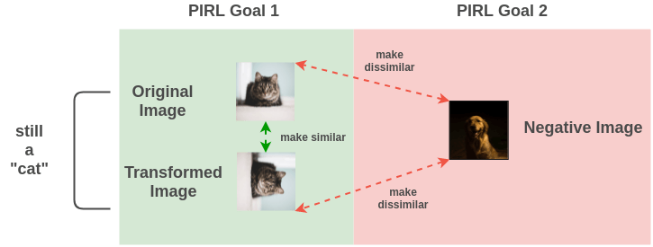
Intuitively this makes sense because even if an image was rotated, it doesn’t change the semantic meaning that this image is still a “cat sitting on a surface”
PIRL Framework
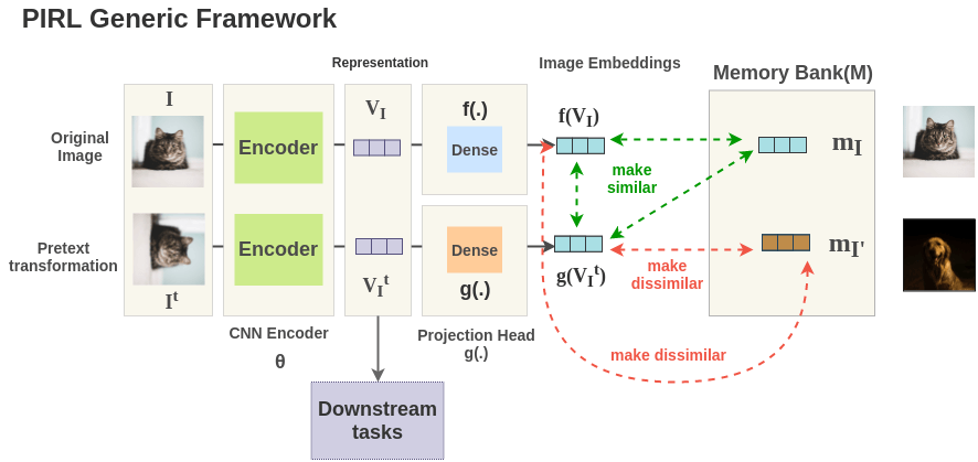
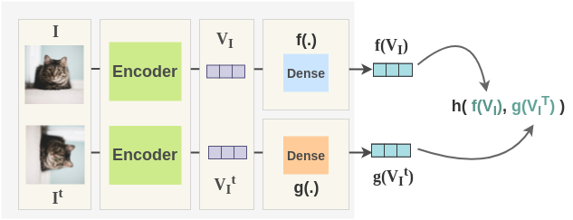
PIRL defines a generic framework to implement this idea. First, you take a original image I, apply a transformation borrowed from some pretext task(e.g. rotation prediction) to get transformed image \(I^t\). Then, both the images are passed through ConvNet \(\theta\) with shared weights to get representations \(V_I\) and \(V_{I^T}\). The representation \(V_I\) of original image is passed through a projection head f(.) to get representation \(f(V_I)\). Similarly, a separate projection head g(.) is used to get representation \(g(V_{I^T})\) for transformed image. These representations are tuned with a loss function such that representations of \(I\) and \(I^t\) are similar, while making it different from other random image representations \(I'\) stored in a memory bank.
Step by Step Example
Let’s assume we have a training corpus containing 3 RGB images for simplicity.
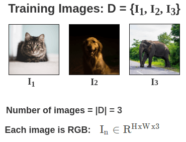
Here is how PIRL works on these images step by step:
- Memory Bank
To learn better image representations, it’s better to compare the current image with a large number of negative images. One common approach is to use larger batches and consider all other images in this batch as negative. However, loading larger batches of images comes with its set of resource challenges.
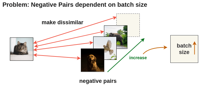
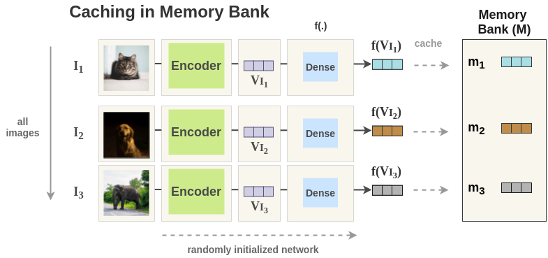
To solve this problem, PIRL proposes to use a memory bank which caches representations of all images and use that during training. This allows us to use a large number of negative pairs without increasing batch size.
In our example, the PIRL model is initialized with random weights. Then, a foward pass is done for all images in training data and the representation \(f(V_I)\) for each image is stored in memory bank.
2. Prepare batches of images
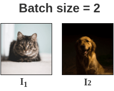
Now, we take mini-batches from the training data. Let’s assume we take a batch of size 2 in our case.
3. Pretext transformation
For each image in batch, we apply the transformation based on the pretext task used. Here, we show the transformation for pretext task of geometric rotation prediction.
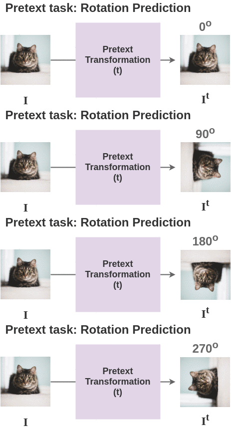
Thus, for 2 images in our batch, we get two pairs and total four images.

4. Encoder
Now, for each image, the image and its counterpart transformation are passed through a network to get representations. The paper uses ResNet-50 as the base ConvNet encoder and we get back 2048-dimensional representation.
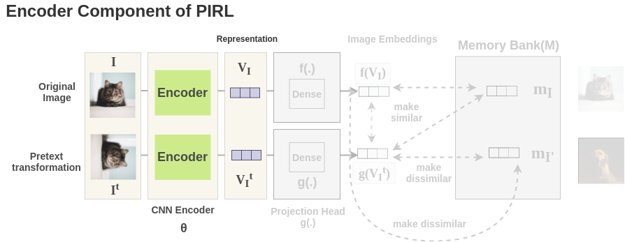
5. Projection Head
The representations obtained from encoder are passed through a single linear layer to project the representation from 2048 dimension to 128 dimension. Separate linear layers f(.) and g(.) are used for the original and transformed image respectively. We get final representation \(f(V_I)\) for original image and \(g(V_{I^T})\) for transformed image.
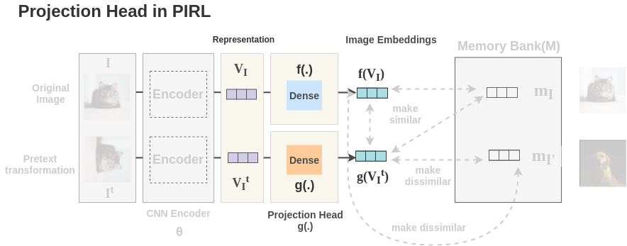
6. Improving Model (Loss function)
Currently, for each image, we have representations for original and transformed versions of it. Our goal is to produce similar representations for both while producing different representations for other images.
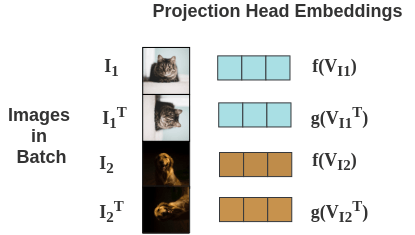
Now, we calculate the loss in the following steps:
a. Cosine Similarity
Cosine similarity is used as a similarity measure of any two representations. Below, we are comparing the similarity of a cat image and it’s rotated counterpart. It is denoted by \(s()\)

- Noise Contrastive Estimator
We use a Noise Contrastive Estimator(NCE) function to compute the similarity score of two representations normalized by all negative images. For a cat image and it’s rotated counterpart, the noise contrastive estimator is denoted by:
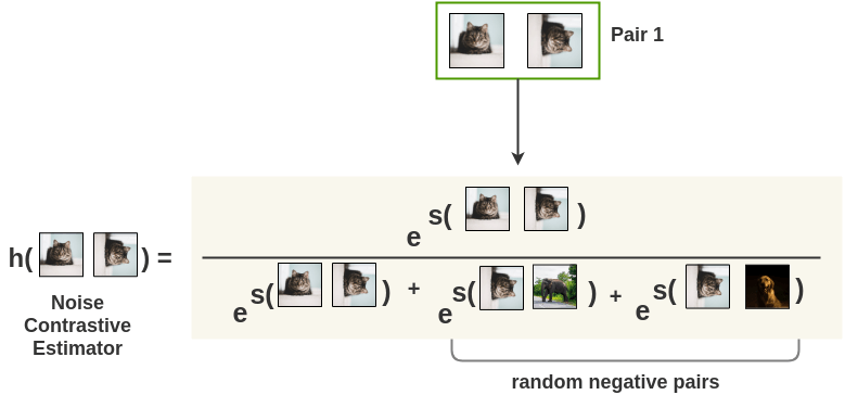
Mathematically, we compute NCE over representations from the projection heads instead of representations from ResNet-50. The formulation is:
\[ h(f(V_I), g(V_{I^T})) = \frac{ exp(\frac{s(f(V_I),\ g(V_{I^t}) )}{\tau} ) }{ exp(\frac{s( f(V_{I}),\ g(V_{I^t}) )}{\tau} ) + \sum_{ I' \in D_{N} } exp(\frac{s( g(V_{I^t}),\ f(V_{I'}) )}{\tau} ) } \]
The loss for a pair of images is calculated using cross-entropy loss as:
\[ L_{NCE}(I, I^t) = -log[h(f(V_I), g(V_{I^t}))] - \sum_{I' \in D_N} log[ 1 - h( g(V_{I^t}), f(V_{I'}) ) ] \]
Since we already have representation of image and negative images in memory bank, we use that instead of computed representation as:
\[ L_{NCE}(I, I^t) = -log[h(m_I, g(V_{I^t}))] - \sum_{I' \in D_N} log[ 1 - h( g(V_{I^t}), m_{I'} ) ] \]
where \(f(V_I)\) is replaced by \(m_I\) and \(f(V_{I'})\) is replaced by \(m_{I'}\).
In ideal case, similarity of image and it’s transformation is highest i.e. 1 while similarity with any negative images is zero. So, loss becomes zero in that case.
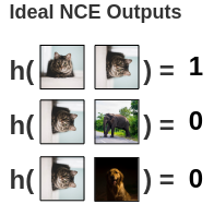
\[ L_{NCE}(I, I^t) = -log[1] - (log[1-0] + log[1-0]) = 0 \]
We see how above loss only compares \(I\) to \(I^t\) and compares \(I^t\) to \(I'\). It doesn’t compare \(I\) and \(I'\). To do that, we introduce another another loss term and combine both these losses using following formulation.
\[ L(I, I^t) = \lambda L_{NCE}(m_I, g(V_{I^t})) + (1-\lambda)L_{NCE}(m_I, f(V_I)) \]
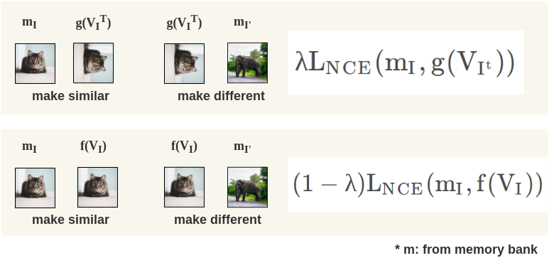
With this formulation, we compare image to its transformation, transformation to negative image and original image to negative image as well.
Based on these losses, the encoder and projection heads improve over time and better representations are obtained. The representations for images in the memory bank for the current batch are also updated by applying exponential moving average.
Transfer Learning
After the model is trained, then the projection heads \(f(.)\) and \(g(.)\) are removed and the ResNet-50 encoder is used for downstream tasks. You can either freeze the ResNet-50 model and use this as a feature extractor or you can finetune the whole network for your downstream task.
Future Work
The authors state two promising areas for improving PIRL and learn better image representations:
1. Borrow transformation from other pretext tasks instead of jigsaw and rotation.
2. Combine PIRL with clustering-based approaches
Code Implementation
An implementation of PIRL in PyTorch by Arkadiusz Kwasigroch is available here. Models are available for both rotation as well as jigsaw task. It tests the performance of the network on a small dataset of 2000 skin lesions images and gets an AUC score of 0.7 compared to a random initialization score of 0.55.
References
Citation
@online{chaudhary2020,
  author = {Chaudhary, Amit},
  title = {The {Illustrated} {PIRL:} {Pretext-Invariant}
    {Representation} {Learning}},
  date = {2020-03-16},
  url = {https://amitness.com/posts/illustrated-pirl.html},
  langid = {en}
}