A Visual Guide to Self-Labelling Images

A self-supervised method to generate labels via simultaneous clustering and representation learning

In the past year, several methods for self-supervised learning of image representations have been proposed. A recent trend in the methods is using Contrastive Learning (SimCLR, PIRL, MoCo) which have given very promising results.

However, as we had seen in our survey on self-supervised learning, there exist many other problem formulations for self-supervised learning. One promising approach is: > Combine clustering and representation learning together to learn both features and labels simultaneously.

A paper Self-Labelling(SeLa) presented at ICLR 2020 by Asano et al. of the Visual Geometry Group(VGG), University of Oxford has a new take on this approach and achieved the state of the art results in various benchmarks.

The most interesting part is that we can auto-generate labels for images in some new domain with this method and then use those labels independently with any model architecture and regular supervised learning methods. Self-Labelling is a very practical idea for industries and domains with scarce labeled data. Let’s understand how it works.

Solving The Chicken and Egg Problem

At a very high level, the Self-Labelling method works as follows:

• Generate the labels and then train a model on these labels
• Generate new labels from the trained model
• Repeat the process

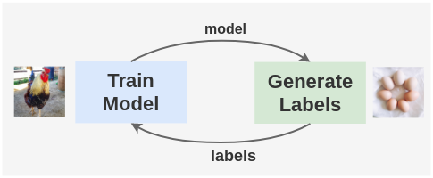
But, how will you generate labels for images in the first place without a trained model? This sounds like the chicken-and-egg problem where if the chicken came first, what did it hatch from and if the egg came first, who laid the egg?

The solution to the problem is to use a randomly initialized network to bootstrap the first set of image labels. This has been shown to work empirically in the DeepCluster paper.

The authors of DeepCluster used a randomly initialized AlexNet and evaluated it on ImageNet. Since the ImageNet dataset has 1000 classes, if we randomly guessed the classes, we would get an baseline accuracy of 1/1000 = 0.1%. But, a randomly initialized AlexNet was shown to achieve 12% accuracy on ImageNet. This means that a randomly-initialized network possesses some faint signal in its weights.

Thus, we can use labels obtained from a randomly initialized network to kick start the process which can be refined later.

Self-Labelling Pipeline

Let’s now understand how the self-labelling pipeline works.

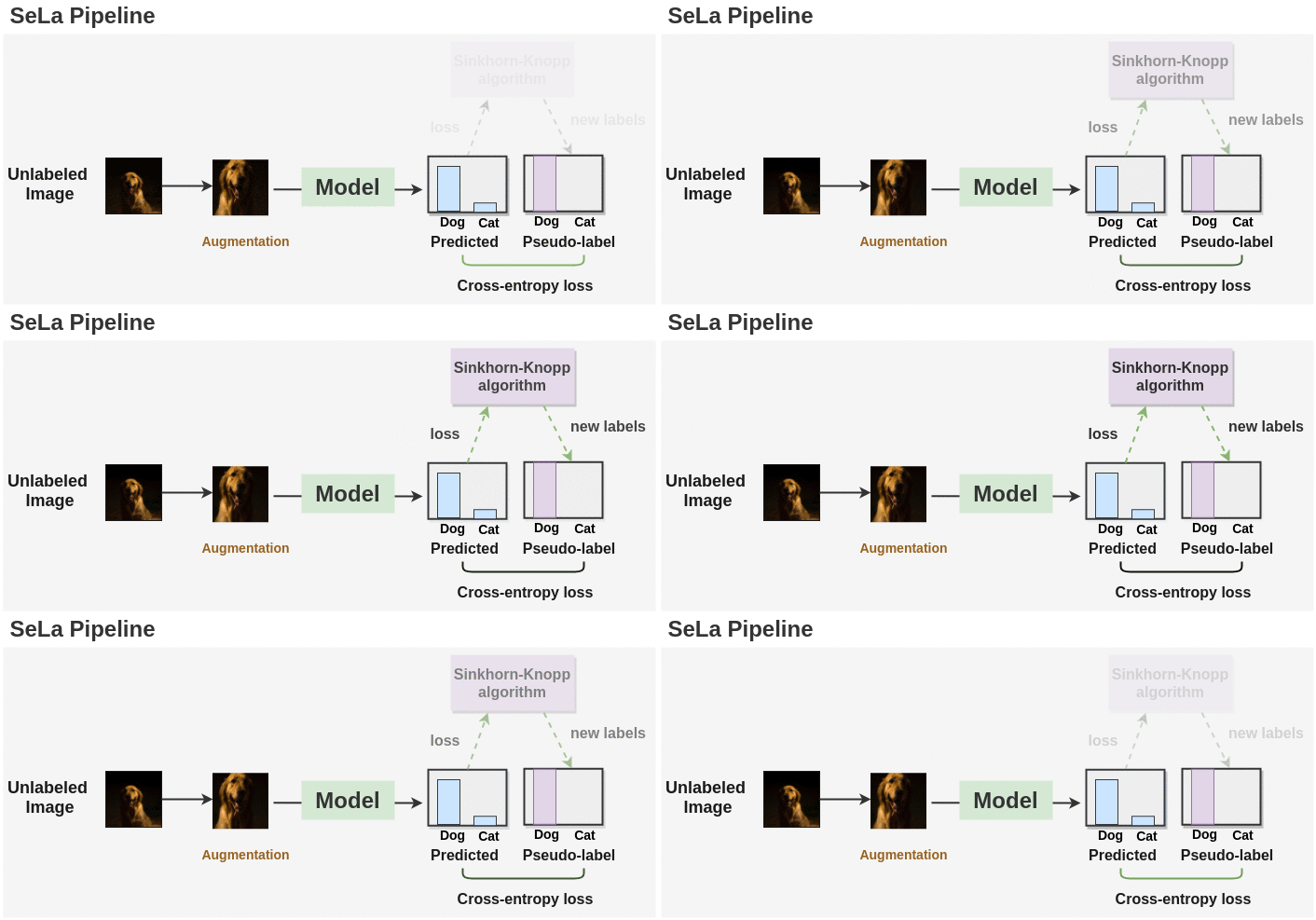
Synopsis:

As seen in the figure above, we first generate labels for augmented unlabeled images using a randomly initialized model. Then, the Sinkhorn-Knopp algorithm is applied to cluster the unlabeled images and get a new set of labels. The model is again trained on these new set of labels and optimized with cross-entropy loss. Sinkhorn-Knopp algorithm is run once in a while during the course of training to optimize and get new set of labels. This process is repeated for a number of epochs and we get the final labels and a trained model.

Step by Step Example

Let’s see how this method is implemented in practice with a step by step example of the whole pipeline from the input data to the output labels:

1. Training Data

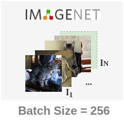
First of all, we get N unlabeled images \[I_1, ..., I_N\] and take batches of them from some dataset. In the paper, batches of 256 unlabeled images are prepared from the ImageNet dataset.

2. Data Augmentation
We apply augmentations to the unlabeled images so that the self-labelling function learned is transformation invariant. The paper first randomly crops the image into size 224*224. Then, the image is converted into grayscale with a probability of 20%. Color Jitter is applied to this image. Finally, the horizontal flip is applied 50% of the time. After the transformations are applied, the image is normalized with a mean of[0.485, 0.456, 0.406] and a standard deviation of [0.229, 0.224, 0.225].

This can be implemented in PyTorch for some image as:

import torchvision.transforms as transforms
from PIL import Image

im = Image.open('cat.png')
aug = transforms.Compose([
    transforms.RandomResizedCrop(224),
    transforms.RandomGrayscale(p=0.2),
    transforms.ColorJitter(0.4, 0.4, 0.4, 0.4),
    transforms.RandomHorizontalFlip(),
    transforms.ToTensor(),
    transforms.Normalize(mean=[0.485, 0.456, 0.406],
                         std=[0.229, 0.224, 0.225])
])
aug_im = aug(im)

3. Choosing Number of Clusters(Labels)

We then need to choose the number of clusters(K) we want to group our data in. By default, ImageNet has 1000 classes so we could use 1000 clusters. The number of clusters is dependent on the data and can be chosen either by using domain knowledge or by comparing the number of clusters against model performance. This is denoted by:

\[ y_1, ..., y_N \in {1, ..., K} \]

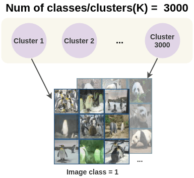
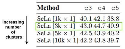
The paper experimented with the number of clusters ranging from 1000(1k) to 10,000(10k) and found the ImageNet performance improves till 3000 but slightly degrades when using more clusters than that. So the papers use 3000 clusters and as a result 3000 classes for the model.

4. Model Architecture
A ConvNet architecture such as AlexNet or ResNet-50 is used as the feature extractor. This network is denoted by \(\color{#885e9c}{\phi(} I \color{#885e9c}{)}\) and maps an image I to feature vector \(m \in R^D\) with dimension D.

Then, a classification head is used which is simply a single linear layer that converts the feature vectors into class scores. These scores are converted into probabilities using the softmax operator.

\[ p(y=.|x_i) = softmax( \color{#3b6eb5}{h\ o\ \phi(}x_i \color{#3b6eb5}{)} ) \]

5. Initial Random Label Assignment
The above model is initialized with random weights and we do a forward pass through the model to get class predictions for each image in the batch. These predicted classes are assumed as the initial labels.

6. Self Labelling with Optimal Transport
Using these initial labels, we want to find a better distribution of images into clusters. To do that, the paper uses a novel approach quite different than K-means clustering that was used in DeepCluster. The authors apply the concept of optimal transport from operations research to tackle this problem.

Let’s first understand the optimal transport problem with a simple real-world example:

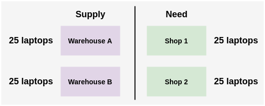
• Suppose a company has two warehouses A and B and each has 25 laptops in stock. Two shops in the company require 25 laptops each. You need to decide on an optimal way to transport the laptops from the warehouse to the shops.

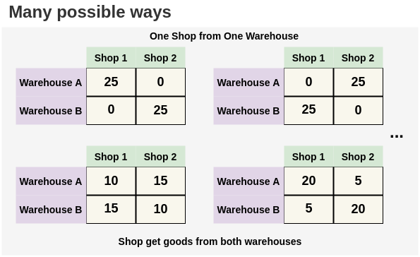
• There are multiple possible ways to solve this problem. We could either assign all laptops from warehouse A to shop 1 and all laptops from warehouse B to shop 2. Or we could switch the shops. Or we could transfer 15 laptops from warehouse A and remaining 10 from warehouse B. The only constraint is that the number of laptops allocated from a warehouse cannot exceed their current limit i.e. 25.

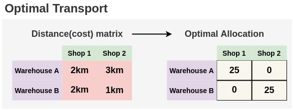
• But, if we know the distance from each warehouse to the shops, then we can find an optimal allocation with minimal travel. Here, we can see intuitively that the best allocation would be to deliver all 25 laptops from warehouse B to shop 2 since the distance is less than warehouse A. And we can deliver the 25 laptops from warehouse A to shop 1. Such optimal allocation can be found out using the Sinkhorn-Knopp algorithm.

Now, that we understand the problem, let’s see how it applies in our case of cluster allocation. The authors have formulated the problem of assigning the unlabeled images into clusters as an optimal transport problem in this way:

1. Problem:
   Generate an optimal matrix Q that allocates N unlabeled images into K clusters.

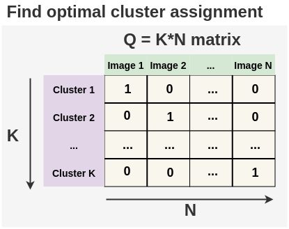
2. Constraint:
   The unlabeled images should be divided equally into the K clusters. This is referred to as the equipartition condition in the paper.

3. Cost Matrix:
   The cost of allocating each image to a cluster is given by the model performance when trained using these clusters as the labels. Intuitively, this means the mistake model is making when we assign an unlabeled image to some cluster. If it is high, then that means our current label assignment is not ideal and so we should change it in the optimization step.

We find the optimal matrix Q using a fast-variant of the Sinkhorn-Knopp algorithm. This algorithm involves a single matrix-vector multiplication and scales linearly with the number of images N. In the paper, they were able to reach convergence on ImageNet dataset within 2 minutes when using GPU to accelerate the process. For the algorithm and derivation of Sinkhorn-Knopp, please refer to the Sinkhorn Distances paper. There is also an excellent blogpost by Michiel Stock that explains Optimal Transport ¹.

7. Representation Learning
Since we have updated labels Q, we can now take predictions of the model on the images and compare it to their corresponding cluster labels with a classification cross-entropy loss. The model is trained for a fixed number of epochs and as the cross-entropy loss decrease, the internal representation learned improves.

\[ E(p|y_1, ..., y_N) = -\frac{1}{N} \sum_{i=1}^{N} logp(y_i \mid x_i) \]

8. Scheduling Cluster Updates
The optimization of labels at step 6 is scheduled to occur at most once an epoch. The authors experimented with not using self-labelling algorithm at all to doing the Sinkhorn-Knopp optimization once per epoch. The best result was achieved at 80.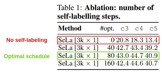

This shows that self-labeling is giving us a significant increase in performance compared to no self-labeling (only random-initialization and augmentation).

Label Transfer

The labels obtained for images from self-labelling can be used to train another network from scratch using standard supervised training.

In the paper, they took labels assigned by SeLa with AlexNet and retrained another AlexNet network from scratch with those labels using only 90-epochs to get the same accuracy.

They did another interesting experiment where 3000 labels obtained by applying SeLa to ResNet-50 was used to train AlexNet model from scratch. They got 48.4% accuracy which was higher than 46.5% accuracy obtained by training AlexNet from scratch directly. This shows how labels can be transferred between architectures.

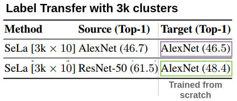
The authors have published their generated labels for the ImageNet dataset. These can be used to train a supervised model from scratch.

• Pseudo-labels from best AlexNet model on ImageNet: alexnet-labels.csv
  
• Pseudo-labels from best ResNet model on ImageNet: resnet-labels.csv

The author have also setup an interactive demo here to look at all the clusters found from ImageNet.

Insights and Results

1. Small Datasets: CIFAR-10/CIFAR-100/SVHN
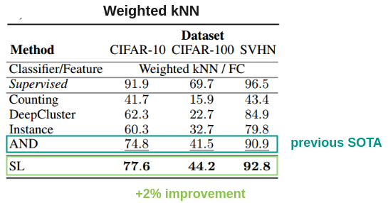
The paper got state of the art results on CIFAR-10, CIFAR-100 and SVHN datasets beating best previous method AND. An interesting result is very small improvement(+0.8%) on SVHN, which the authors say is because the difference between supervised baseline of 96.1 and AND’s 93.7 is already small (<3%).

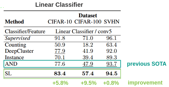
The authors also evaluated it using weighted KNN and an embedding size of 128 and outperformed previous methods by 2%.

2. What happens to equipartition assumption if the dataset is imbalanced?
The paper has an assumption that images are equally distributed over classes. So, to test the impact on the algorithm when it’s trained on unbalanced datasets, the authors prepared three datasets out of CIFAR-10:

• Full: Original CIFAR-10 dataset with 5000 images per class
• Light Imbalance: Remove 50% of images in the truck class of CIFAR-10
• Heavy Imbalance: Remove 10% of first class, 20% of second class and so on from CIFAR-10

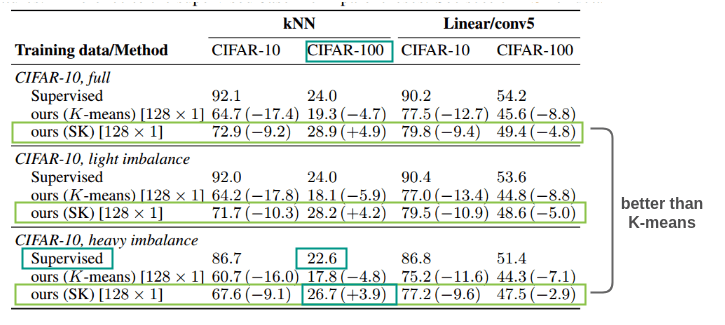
When evaluated using linear probing and kNN classification, SK(Sinkhorn-Knopp) method beat K-means on all three conditions. In light imbalance, no method was affected much. For heavy imbalance, all methods dropped in performance but the performance decrease was lower for self-supervised methods using k-means and self-labelling than supervised ones. The self-labelling method beat even supervised method on CIFAR-100. Thus, this method is robust and can be applied for an imbalanced dataset as well.

Code Implementation

The official implementation of Self-Labelling in PyTorch by the paper authors is available here. They also provide pretrained weights for AlexNet and Resnet-50.

References

• Self-labelling via simultaneous clustering and representation learning
• Deep Clustering for Unsupervised Learning of Visual Features
• Visual Geometry Group Blog, University of Oxford

Footnotes

1. https://michielstock.github.io/OptimalTransport/